Neural ODE from scratch and revisit backward propagation
Neural Network is a powerful tool as a universal functional approximator and plays a vital role in Deep Learning. To boost the performance on various task, researchers add prior knowledge to the network on different tasks, for example, using Convolutional Neural Neural network on image recognition and Recurrent Network on sequence model. In NIPS 2018, researchers from University of Toronto propose a new Neural network architecture:
Neural Ordinary Differential Equations
and received the best paper award.
I spent some time trying to understand the nitty-gritty details of Neural ODE and reproduce the results. I did it as an exercise and decided to write a post about it (full code here). This blog intends to go through the details, intuition and tricks to implement it with PyTorch. Most of the code reference from Mikhail Surtsukov excellent blog post and the original paper.
Prerequisites
I strongly advise reader go through part 1, part 2, appendix A, B, C in the original paper first, which this blog focus on to elaborate. Nevertheless, you will need the following knowledge to understand the material.
- Basic understanding of calculus and differential equations.
- Basic understanding of Neural Network and backward propagation
- Basic understanding of Python and Pytorch
Why ODE (Ordinary Differential Equations)?
Many dynamical systems are more natural to described using ODE. For example, population, epidemic (like COVID-19), and especially physics and engineering. It is natural to learn the dynamics instead of the observable, which could be hard to understand and describe. (especially for physics and control theory). For example, to describe a simple harmonic motion:
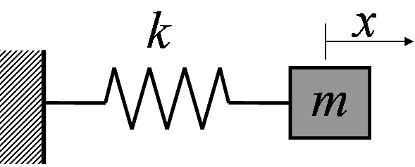
We can write down the Equation of Motion (EOM) in terms of ODE.


We can see the differential equation is just linear equation(s) and the solution is in a more complex form. It is very natural to model the interested system in terms of differential equations.
General Idea of training the Neural ODE
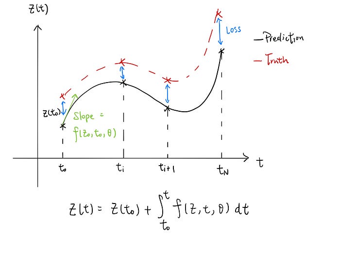
The idea is simple and just like ordinary supervised learning
- Solve the Neural ODE with some initial value
- compare the path with the true label and compute the loss
- minimise the loss
Let’s start by solving the Neural ODE
We can solve the following ODE

by integrating along the path

In practice, we don’t want to calculate the analytic form of the ODE (can we ?) so instead of integrating the function, we can get z(t) with numerical approximation.
There are lots of numerical methods to solve the differential equation, and we use the simplest one here, the Euler Method. The idea is simple. Instead of doing it in infinitesimal steps, we approximate the solutions with small discrete time steps.
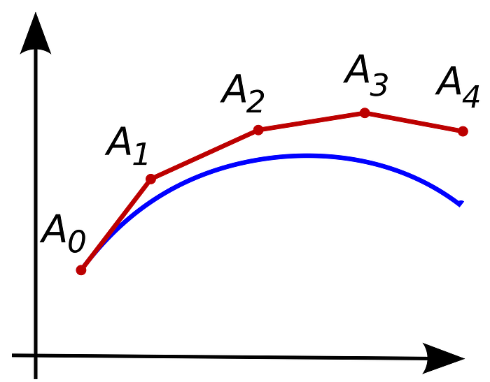
Now we can create our first python function to solve the ODE given the initial value, the ODE function, and find the trajectory in later time step.
def ode_solve(z0, t0, t1, f):
    """
    Simple Euler ODE initial Value solver
    :param z0: initial value
    :param t0: initial time stamp
    :param t1: target time stamp
    :param f: ODE function
    :return: z1
    """
    h_max = 0.05
    n_steps = math.ceil((abs(t1 - t0) / h_max).max().item())

    h = (t1 - t0) / n_steps
    t = t0
    z = z0

    for i_step in range(n_steps):
        z = z + h * f(z, t)
        t = t + h
    return z
Next we need to compute the loss.
Compute the loss function
Computing the loss is easy. By looking at figure 1, we can calculate the loss by just calculating the distance between the outputs and the labels. It can be done using mean square error. For example, in PyTorch we can use the following function.
loss = F.mse_loss(outputs, labels.detach())After that, we can use standard optimisation technique to minimise the loss. The standard one for differentiable functions is gradient descent, and we can compute the gradient with backward propagation.
How do we do backward propagation?
For an ordinary neural network, we know how to do backward propagation to each neuron and parameters.
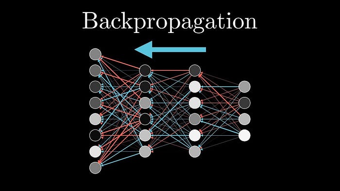
We can certainly do it on the numerical integrator, but it will introduce high memory cost and numerical error. On the other hand, we can assume that we are doing it on the “Correct path” with infinitesimal step, and compute the gradient irrespective of the integration we use.
But how do we do backpropagation on a continuous path? The loss w.r.t. to parameters will also be continuous, and how do we compute it?
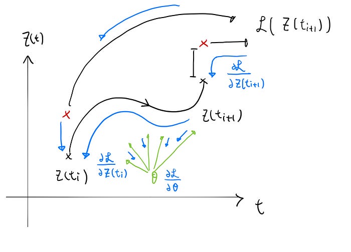
The original authors use the adjoint sensitive method which solves the problem and provides proofs in the appendix. I will explain a little bit more on the details and proof following the author’s approach.
Continuous Backward Propagation
First, imagine we treat two near points as two separate nodes with share parameters:
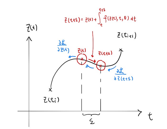
Now we can do backward propagation using chain rules:

for ease of notation: we write the partial derivatives as follow

Instead of computing the partial derivatives directly, we find the “Change in partial derivatives” by taking limit from discrete case to continuous case.
following proof from the original paper:

Notice by taking the limit to 0, we can use the definition of derivative to get another ODE to describe how errors are being backpropagated w.r.t. z(t). It is defined as the adjoint differential equation.
Important implementation detail
The above equation describes the “error dynamic” for between two points on the curve. To accommodate for all pairs, we need to adjust the error by calculating the total change. (notice why there’s 0+ in the limit?) If this is not obvious to the reader (which happens to me), we can compare the computational graph in the discrete case.

Using this method, we can compute the partial derivative of loss w.r.t every point on the curve.
Now we need the gradient of the parameters
It puzzles me for a long time since every point of the curve still contribute to derivative w.r.t. the parameters.

My first intuition is to find:

which is hard to compute without the explicit form of z(t).
The original paper proposed a brilliant method to tackle the problem. Instead of treating the parameters as constant to the dynamics / ODE. We treat it as part of the dynamic! We construct an augmented ODE:

which treat

Now by following the above proof again, replacing

We have

Parts of the Jacobian are known since we know the “dynamic” of θ and t.

now we can obtain the adjoint differential equation for all variable of the differential equations.

Now all we need is the initial points, and we can use any ODE solver to solve

So what does these equation means?
I found it fuzzy to understand the following partial derivatives

I spent some time digesting the meaning, and I found the following way is easier to understand and picture the equation.
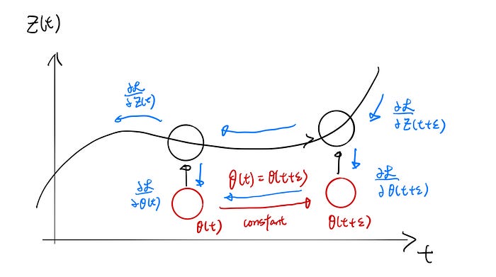
Unlike figure 4, which every z(t) depends on θ, we treat the parameters as a constant “function” in time.

Now observe from figure 6 (blue arrow) that

mean the total derivatives at time t. When we back propagation through time, we obtain the the “total error” from the “final time step” to current time t. If we go back all the way to the starting point, we obtain the total derivatives.
In the continuous case, we only need to find

and we will obtain the total partial derivative of the loss function w.r.t. the parameters.
How do we find the initial value?
To find the initial value for the adjoint differential equation, we can use chain rule starting from the loss function.
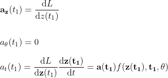
I cannot find a very satisfying way to set the initial value to zero for the adjoint differential equation for the parameters, nevertheless here’s how I picture it.
- θ(t_1) can only contribute an infinitesimal amount to the loss so we can set it to zero
- by solving the initial value problem, the initial value contributes to a constant shift to the final output only. We can don’t need to find the
If anyone has a better explanation, please let me know!
Backward Propagation summary:


By solving the adjoint differential equation using any ODE solver, we can perform continuous backward propagation.
Important methods in PyTorch
I am not going into every detail in the code. Interested audience can find it here. There are a few important parts that I will cover here which relate to the theory described above.
First, How to compute the adjoint differential equation at time t
Since the adjoint differential equation requires partial derivative to the ODE function, the easiest way is to use autograd to find the derivatives.

out = self.forward(z, t)
# direction for autograd
a = grad_outputs

adfdz, adfdt, *adfdp = torch.autograd.grad(
    (out,)
    , (z, t) + tuple(self.parameters())
    , grad_outputs=(a)
    , allow_unused=True
    , retain_graph=True
)
Now notice in torch.autograd.grad() we have an option to choose the output direction. If we use the adjoint state as direction, PyTorch automatically gives us the augmented dynamic we want.
Custom PyTorch function to perform forward and backward propagation
For autograd to work its magic by just calling
loss.backward()We need to have a way to automate the forward pass and backward pass irrespective of the ODE solver.
We can define function with custom forward and backward using
torch.autograd.Functionwhich takes in the Neural ODE model
funcIn forward pass, it simply means solving the Neural ODE function IVP.
@staticmethod
def forward(ctx, z0, t, flat_parameters, func):
    bs, *z_shape = z0.size()
    time_len = t.size(0)

    with torch.no_grad():
        z = torch.zeros(time_len, bs, *z_shape).to(z0)
        z[0] = z0
        for i_t in range(time_len - 1):
            z0 = ode_solve(z0, t[i_t], t[i_t+1], func)
            z[i_t+1] = z0

    ctx.func = func
    ctx.save_for_backward(t, z.clone(), flat_parameters)
    return z
We can see there’s for loop to generate the trajectory using ode_solve with the Nerual ODE (func). ctx is an object that save useful information for backward pass.
Now for the custom backward function:
@staticmethod
def backward(ctx, dLdz):

    func = ctx.func
    t, z, flat_parameters = ctx.saved_tensors
    time_len, bs, *z_shape = z.size()
    n_dim = np.prod(z_shape)
    n_params = flat_parameters.size(0)

    def augmented_dynamics(aug_z_i, t_i):
        ...
        return torch.cat((func_eval, -adfdz, -adfdp, -adfdt), dim=1)

    dLdz = dLdz.view(time_len, bs, n_dim)

    with torch.no_grad():
        adj_z = torch.zeros(bs, n_dim).to(dLdz)
        adj_p = torch.zeros(bs, n_params).to(dLdz)
        adj_t = torch.zeros(time_len, bs, 1).to(dLdz)

        for i_t in range(time_len-1, 0, -1):
            z_i = z[i_t]
            t_i = t[i_t]
            f_i = func(z_i, t_i).view(bs, n_dim)

            dLdz_i = dLdz[i_t]
            a_t = torch.transpose(dLdz_i.unsqueeze(-1), 1, 2)
            dLdt_i = -torch.bmm(a_t, f_i.unsqueeze(-1))[:, 0]

            adj_z += dLdz_i
            adj_t[i_t] = adj_t[i_t] + dLdt_i

            aug_z = torch.cat((z_i.view(bs, n_dim), adj_z, torch.zeros(bs, n_params).to(z), adj_t[i_t]), dim=-1)

            aug_ans = ode_solve(aug_z, t_i, t[i_t-1], augmented_dynamics)

            adj_z[:] = aug_ans[:, n_dim:2*n_dim]
            adj_p[:] += aug_ans[:, 2*n_dim:2*n_dim + n_params]
            adj_t[i_t-1] = aug_ans[:, 2*n_dim + n_params:]

            del aug_z, aug_ans

        ## Adjust 0 time adjoint with direct gradients
        # Compute direct gradients
        dLdz_0 = dLdz[0]
        dLdt_0 = -torch.bmm(torch.transpose(dLdz_0.unsqueeze(-1), 1, 2), f_i.unsqueeze(-1))[:, 0]

        # Adjust adjoints
        adj_z += dLdz_0ri
        adj_t[0] = adj_t[0] + dLdt_0
    # forward: (z0, t, parameters, func)
    return adj_z.view(bs, *z_shape), adj_t, adj_p, None
I strongly advice interested reader go through the code by themselves since the dimension of each vector are not shown in the code. It is essential to go through the details for it to work. Things that I want to highlight in the code.
- Remember to adjust the gradient at each data point. The gradient contributes from both the path and the loss refer to the above figures.
- The augmented dynamic, and adjoint state computation follows the algorithm from appendix C.
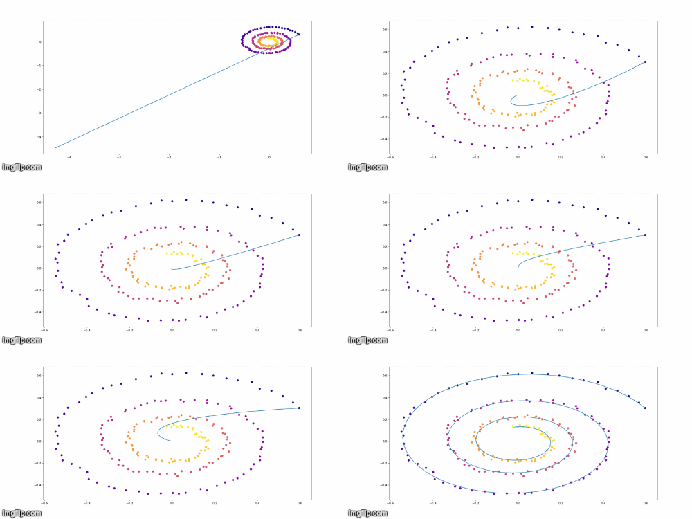
Training Example on Toy Model
Conclusion
I started this exercise since I want to understand the details of Neural ODE and the best way to do it is code it out! This post focuses more on the derivation, implementation details and miss a lot of things from the original paper. For example, how to use it as a residual block in solving MNIST, generative model, and various experiment results. I strongly advise checking the original paper and presentation from the authors for more details.
